ggplot2高级:构建自己的图层

这部分内容是Extending ggplot2的学习笔记，大部分内容都是原文的简单翻译。

所有的ggplot2对象都建立自”ggproto”这套面向对象编程系统，因此想要创建出自己的一套图层，而不是简单的对已有图层进行累加，那么就需要学习”ggproto”。

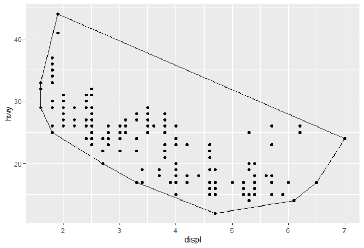
创建新的stat

最简单的stat

我们会从一个最简单的stat开始: 根据已有的一组点，用一个凸壳(convex hull)包围他。

第一步，我们创建一个继承自Stat的”ggproto”对象

StatChull <- ggproto("StatChull", Stat,
                     compute_group = function(data, scales){
                       data[chull(data$x, data$y), , drop=FALSE]
                     },
                     required_aes = c("x","y")
)

在”ggproto”函数中，前两个是固定项，分别是类名和继承的”ggproto”类。而后续内容则是和你继承的类相关，例如compute_group()方法负责计算，required_aes则列出哪些图形属性(aesthetics)必须要存在，这两个都继承自Stat，可以用?Stat查看更多信息。。

第二步，我们开始写一个图层。由于历史设计原因，Hadley将其称作stat_()或geom_()。但实际上，Hadley认为layer_()可能更准确些，毕竟每一个图层都或多或少的有”stat”和”geom”。

所有的图层都遵循相同的格式，即你在function中声明默认参数，然后调用layer()函数，将...传递给params参数。在...的参数既可以是”geom”的参数(如果你要做一个stat封装)，或者是”stat”的参数(如果你要做geom的封装)，或者是将要设置的图形属性. layer()会小心的将不同的参数分开并确保它们存储在正确的位置:

stat_chull <- function(mapping = NULL, data = NULL, geom = "polygon",
                       position = "identity", na.rm = TRUE, show.legend = NA,
                       inherit.aes = TRUE, ...){
  layer(
    stat = StatChull, data = data, mapping = mapping, geom = geom,
    position = position, show.legend = show.legend, inherit.aes = inherit.aes,
    params = list(na.rm = na.rm, ...)
    
  )
}

(注, 在写R包的时候要注意用ggplot2::layer()或在命名空间中导入layer(), 否则会因找到函数而报错)

当我们写好了图层函数后，我们就可以尝试这个新的”stat”了

ggplot(mpg, aes(displ, hwy)) +
  geom_point() +
  stat_chull(fill = NA, colour= "black")

(后续我们会学习如何通过设置”geom”的默认值，来避免声明fill=NA)

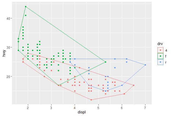
一旦我们构建了这种基本的对象，ggplot2将会给我们带来极大的自由。举个例子，ggplot2自动保留每组中不变的图形属性，也就是说你可以分组绘制一个凸壳:

ggplot(mpg, aes(displ, hwy, colour = drv)) + 
  geom_point() + 
  stat_chull(fill = NA)

我们还可以覆盖默认的图层，来以不同的形式展现凸壳:

ggplot(mpg, aes(displ, hwy)) +
  stat_chull(geom = "point", size = 4, colour = "red") +
  geom_point()

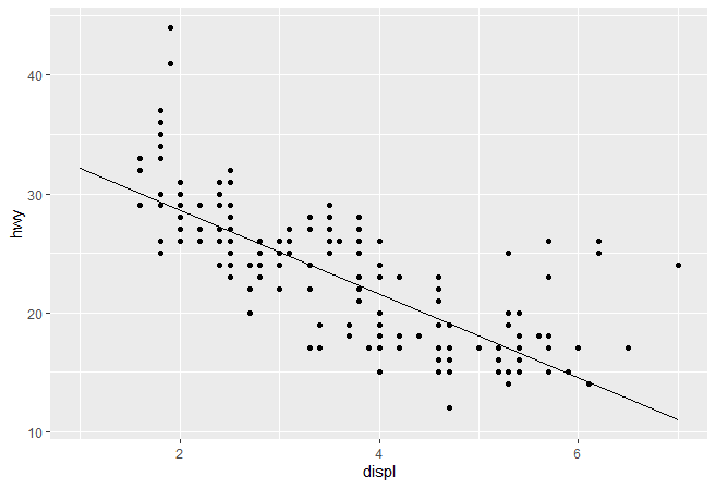
Stat参数

一个更加复杂的”stat”会做一些计算。我们可以通过实现一个简单版本的geom_smooth来了解。我们将会创建一个新的图层StatLm（继承自Stat）和一个的图层函数stat_lm():

# 基于ggproto创建StatLm
StatLm <- ggproto("StatLm", Stat,
                  required_aes = c("x", "y"),
                  compute_group = function(data, scales){
                    rng <- range(data$x, nr.rm = TRUE)
                    grid <- data.frame(x = rng)
                    mod <- lm(y ~ x, data = data)
                    grid$y <- predict(mod, newdata = grid)
                    grid
                  }
                  )
# 创建图层函数
stat_lm <- function(mapping = NULL, data = NULL, geom = "line",
                    position = "identity", na.rm = FALSE, show.legend = NA,
                    inherit.aes = TRUE, ...){
  layer(
    stat = StatLm, data = data, mapping = mapping, geom = geom,
    position = position, show.legend = show.legend, inherit.aes = inherit.aes,
    params = list(na.rm = na.rm, ...)
  )
}

调用我们写的stat_lm()图形，检查下效果

ggplot(mpg, aes(displ, hwy)) + 
  geom_point() + 
  stat_lm()

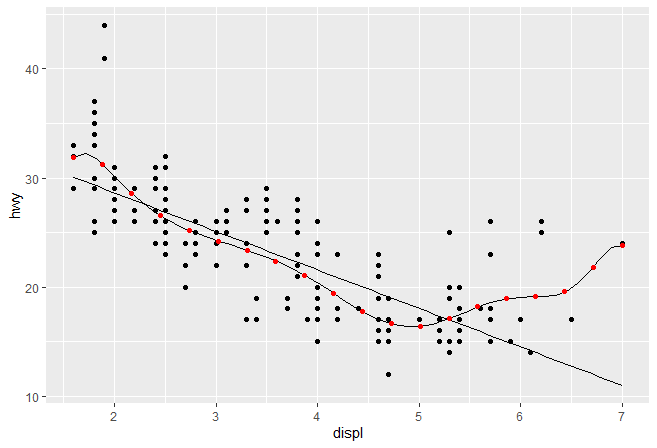
StatLm缺少参数不太灵活，只能做单一线性拟合。最好是允许用户能够自由修改模型公式和创建图层所需要的数据量。为了实现这一需求，我们在compute_group()增加了一些参数，代码如下:

# 增加了参数n和formula
StatLm2 <- ggproto("StatLm2", Stat,
                  required_aes = c("x", "y"),
                  compute_group = function(data, scales, params, 
                                           n = 100, formula = y ~x){
                    
                    rng <- range(data$x, na.rm = TRUE)
                    grid <- data.frame(x = seq(rng[1], rng[2],length = n))
                    
                    mod <- lm(formula, data = data)
                    grid$y <- predict(mod, newdata = grid)
                    grid
                  })
# 固定模板
stat_lm2 <- function(mapping = NULL, data = NULL, geom = "line",
                     position = "identity", na.rm = TRUE, show.legend = NA,
                     inherit.aes = TRUE, n = 50, formula = y ~ x,
                     ...){
  layer(stat = StatLm2, data = data, mapping = mapping, geom = geom,
        position = position, show.legend = show.legend, inherit.aes = inherit.aes,
        params = list( n = n, formula = formula, na.rm = na.rm, ...))
}
# 绘图
ggplot(mpg, aes(displ, hwy)) + 
  geom_point() + 
  stat_lm() +
  stat_lm2(formula = y ~ poly(x, 10)) +
  stat_lm2(formula = y ~ poly(x, 10), geom = "point", colour = "red", n =20)

我们并不需要显式在图层中包括新的参数，..会将这些参数放到合适的地方。但是你必须在文档中写出哪些参数是可以让用户调整的，以便用户知道他们的存在。举个一个简单的例子

#' @export
#' @inheritParams ggplot2::stat_identity
#' @param formula The modelling formula passed to \code{lm}. Should only 
#'   involve \code{y} and \code{x}
#' @param n Number of points used for interpolation.
stat_lm <- function(mapping = NULL, data = NULL, geom = "line",
                    position = "identity", na.rm = FALSE, show.legend = NA, 
                    inherit.aes = TRUE, n = 50, formula = y ~ x, 
                    ...) {
  layer(
    stat = StatLm, data = data, mapping = mapping, geom = geom, 
    position = position, show.legend = show.legend, inherit.aes = inherit.aes,
    params = list(n = n, formula = formula, na.rm = na.rm, ...)
  )
}

上面代码中以#' 开头内容都是roxygon语法，其中@inheritParams ggplot2::stat_identity表示在最后输出的帮助文档中会继承stat_identity的参数说明。而@export则是将函数让用户可见，否则用户无法直接调用。

挑选参数

有些时候，你会发现部分运算是针对所有数据集进行，而非每个分组。比较好的方法就是挑选明智的默认值。例如，我们需要做密度预测，我们有理由为整个图形挑选一个带宽(bandwidth)。下面的”Stat”创建了stat_density()的变体，通过选择每组最优带宽的均值作为所有分组的带宽。

StatDensityCommon <- ggproto("StatDensityComon", Stat,
                             required_aes = "x",
                             
                             setup_params = function(data, params){
                               if (!is.null(params$bandwidth))
                                 return(params)
                               
                               xs <- split(data$x, data$group)
                               bws <- vapply(xs, bw.nrd0, numeric(1))
                               bw <- mean(bws)
                               message("Picking bandwidth of ", signif(bw,3))
                               
                               params$bandwidth <- bw
                               params
                               },
                             
                             compute_group = function(data, scales, bandwidth = 1){
                               d <- density(data$x, bw = bandwidth)
                               data.frame(x = d$x, y = d$y)
                               
                             }
                             )

stat_density_common <- function(mapping = NULL, data = NULL, geom = "line",
                                position = "identity", na.rm = FALSE,
                                show.legend = NA, inherit.aes = TRUE,
                                bandwidth = NULL, ...){
  layer(stat = StatDensityCommon, data = data, mapping = mapping,
        geom = geom, position = position, show.legend = show.legend,
        inherit.aes = inherit.aes, 
        params = list(bandwidth = bandwidth, na.rm = na.rm, ...))
}

ggplot(mpg, aes(displ, colour = drv)) +
  stat_density_common()

作者推推荐用NULL作为默认值。如果你通过自动计算的方式挑选了重要参数，那么建议通过message()的形式告知用户(在答应浮点值参数时，用singif()可以只展示部分小数点)。

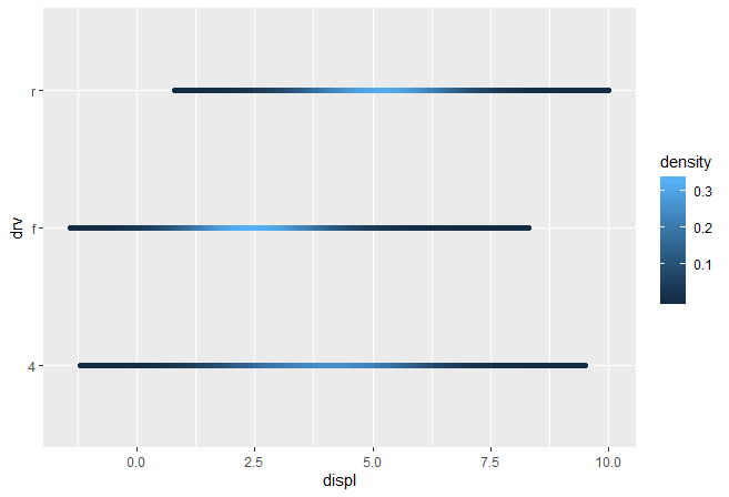
变量名和默认图形属性

这部分”stat”会阐述另外一个重要的点。当我们想要让当前”stat”对其他geoms更加有用时，我们应该返回一个变量，称之为”density”而不是”y”。之后，我们可以设置”default_aes”自动地将density映射到y, 这允许用户覆盖它从而使用不同的”geom”.

StatDensityCommon <- ggproto("StatDentiy2", Stat,
                             required_aes = "x",
                             default_aes = aes(y = stat(density)),
                             
                             compute_group = function(data, scales, bandwidth = 1){
                               d <- density(data$x, bw= bandwidth)
                               data.frame(x = d$x , density=d$y)
                             }
                             )
ggplot(mpg, aes(displ, drv, colour = stat(density))) +
  stat_density_common(bandwidth = 1, geom="point")

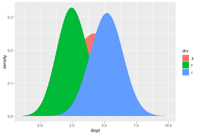
然而直接在stat中用area geom的结果可能和你想的不同。

ggplot(mpg, aes(displ, fill = drv)) + 
  stat_density_common(bandwidth = 1, geom = "area", position = "stack")

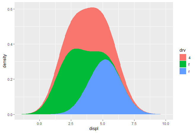
密度不是一个相互累加，而是单独计算，因此预测的x没有对齐。我们可以通过在setup_params()计算数据范围的方式解决该问题

StatDensityCommon <- ggproto("StatDensityCommon", Stat, 
  required_aes = "x",
  default_aes = aes(y = stat(density)),

  setup_params = function(data, params) {
    min <- min(data$x) - 3 * params$bandwidth
    max <- max(data$x) + 3 * params$bandwidth
    
    list(
      bandwidth = params$bandwidth,
      min = min,
      max = max,
      na.rm = params$na.rm
    )
  },
  
  compute_group = function(data, scales, min, max, bandwidth = 1) {
    d <- density(data$x, bw = bandwidth, from = min, to = max)
    data.frame(x = d$x, density = d$y)
  }  
)

ggplot(mpg, aes(displ, fill = drv)) + 
  stat_density_common(bandwidth = 1, geom = "area", position = "stack")

使用”raster”几何形状

ggplot(mpg, aes(displ, drv, fill = stat(density))) + 
  stat_density_common(bandwidth = 1, geom = "raster")

练习题

1. 拓展stat_chull，使其能够计算alpha hull, 类似于alphahull. 新的”stat”能够接受alpha做为参数
2. 修改最终版本的StatDensityComon, 使其能够接受用户定义的min和max. 你需要同时修改layer函数和compute_group()方法
3. 将StatLm和ggplot2::StatSmooth对比。是什么差异使得StatSmooth比StatLm更加复杂。

创建新的geom

相对于创建新的”stat”, 创建新的”geom”会将难一些，因为这需要你懂得一些grid知识。因为ggplot2基于grid，所以你得要学一些用grid绘图的知识。如果你真的打算学习如何新增一个新的”geom”，Hadley推荐你买Paul Murrell所著的R绘图系统。里面介绍所有和用”grid”绘图相关的知识。

一个简单的geom

让我们先从一个简单的案例入手，尝试实现一个类似于geom_point()的图层

# ggproto原型
GeomSimplePoint <- ggproto("GeomSimplePoint", Geom,
                           required_aes = c("x","y"),
                           default_aes = aes(shape = 19, size = 0.1, colour = "black"),
                           draw_key = draw_key_point,
                           
                           draw_panel = function(data, panel_params, coord){
                             coords <- coord$transform(data, panel_params)
                             grid::pointsGrob(
                               coords$x, coords$y,
                               pch = coords$shape,
                               size = unit(coords$size, "char"),
                               gp = grid::gpar(col=coords$colour)
                             )
                             
                           }
)
# 图层函数
geom_simple_point <- function(mapping = NULL, data = NULL, stat = "identity",
                              position = "identity", na.rm = FALSE, show.legend = NA,
                              inherit.aes = TRUE, ...){
  
  layer(geom = GeomSimplePoint, mapping = mapping, data = data, stat = stat,
        position = position, show.legend = show.legend, inherit.aes = inherit.aes,
        params = list(na.rm = na.rm, ...))
}                       

ggplot(mpg, aes(displ, hwy)) + 
  geom_simple_point()

上面的代码和构建新的”stat”非常的相似，我们同样需要为4块内容提供属性/方法

• required_aes: 用户所必需的提供的美术属性
• default_aes: 默认的图形属性值
• draw_key: 提供在图例(legend)绘制关键信息的函数，可用?draw_key查看帮助文档
• draw_panel: 这里就是见证奇迹的地方。该函数接受三个参数作为输入，返回一个grid的”grob”对象。它在每个面板(panel)运行一次。由于它是最复杂的内容，因此我们有必要详细地介绍它。

draw_panel有三个参数

• data: 数据框，每一列都是一个图形属性
• panel_params: 一个列表，里面是coord产生的每个面板的参数。你需要将其当做一个不透明的数据结构: 不要看里面的细节，只要将其传递给coord方法。
• coord: 一个描述坐标系统的对象

你需要共同使用panel_params和coord才能对数据进行转换，即coords <- coord$transform(data, panel_params)。这会创建一个数据框，里面的位置变量会被缩放到0-1之间。得到缩放数据用于调用”grid”的grob函数。(非笛卡尔坐标系统的数据转换比较复杂，你最好是将数据转成已有ggplot2的”geom”所接受的格式，然后传递)。

分组geoms

上一步我们用到的是draw_panel，也就是为每一行元素创建一个图形元素，比如说上面的GeomSimplePoint就是每一行一个点，这是最常见的情况。当然，如果你想为每一个分组绘制一个图形元素，那么我们应该使用draw_group()。

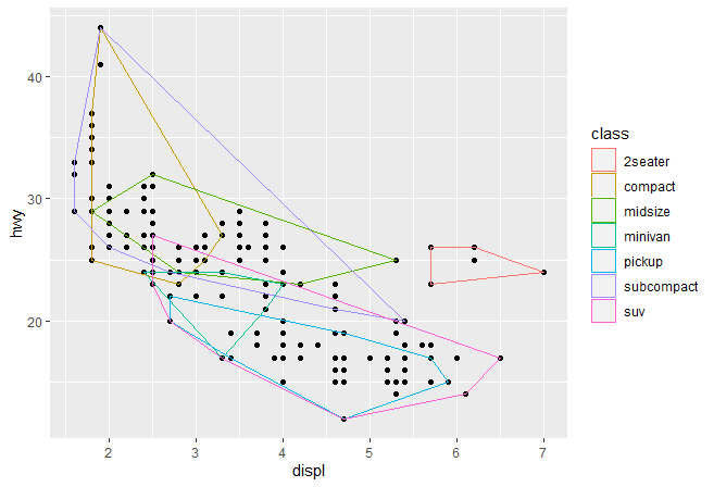
我们用一个简化版的GeomPolygon为例讲解这个知识点:

GeomSimplePolygon <- ggproto("GeomPolygon", Geom,
                             required_aes = c("x", "y"),
                             default_aes = aes(
                               colour = NA, fill = "grey20", size = 0.5,
                               linetype = 1, alpha = 1
                             ),
                             
                             draw_key = draw_key_polygon,
                             
                             draw_group = function(data, panel_params, coord){
                               n <- nrow(data)
                               if (n <= 2) return(grid::nullGrob())
                               
                               coords <- coord$transform(data, panel_params)
                               
                               first_row <- coords[1, , drop = FALSE]
                               
                               grid::polygonGrob(
                                 coords$x, coords$y,
                                 default.units = "native",
                                 gp = grid::gpar(
                                   col = first_row$colour,
                                   fill = scales::alpha(first_row$fill, first_row$alpha),
                                   lwd = first_row$size * .pt,
                                   lty = first_row$linetype
                                 )
                               )                                                          
                             }
                            )

geom_simple_polygon <- function(mapping = NULL, data = NULL, stat = "chull",
                                position = "identity", na.rm = FALSE, 
                                show.legend = NA, inherit.aes = TRUE, ...){
  layer(
    geom = GeomSimplePolygon, mapping = mapping, data = data, stat = stat,
    position = position, show.legend = show.legend, inherit.aes = inherit.aes,
    params = list(na.rm = na.rm, ...)
  )
  
}

ggplot(mpg, aes(displ, hwy)) +
  geom_point() + 
  geom_simple_polygon(aes(colour = class), fill = NA)

这里有几个注意点

• 我们重写了draw_group()而不是draw_panel(), 这是因为我们希望polygon是按照绘制，而不是按行绘制。
• 我们分组数据中不到两行，也就是没有足够的数据点去绘制polygon，因此我们返回了一个nullGrob()。你认为认为这是图形上的NULL: 这是一个grob对象，什么也不画，并且也不占任何空间
• 在单位上，x和y都应该是native的单位。(默认pointGrob()的单位就是native，因此我这里没有做修改)。多边形线的宽度(lwd)取决于点的大小，而ggplot2计算的点大小返回的mm单位结果，因此作者将其和.pt相乘，将其调整为内部lwd接受的输入。

如果你将我们写的和实际的GeomPolygon比较，你会发现后者重写了draw_panel()，这是因为他用了一些小技巧来创建polygonGrob()从而在一次运行中得到多个polygon。这虽然更加复杂，但是在性能上更优秀。

从已有的Geom中继承

有些时候，你只想对已有的图层做一些小的修改。在这种情况下，除了从Geom继承以外，你还可以从已有的子类中继承。举个例子，我们可能想要更改GeomPolygon的默认值，使其更好的在StatChull中工作:

#GeomPolygonHollow继承自GeomPolygon
GeomPolygonHollow <- ggproto("GeomPolyHollwo", GeomPolygon,
                             default_aes = aes(colour = "black", fill = NA,
                                               size = 0.5, linetype = 1, 
                                               alpha = NA))
# layer的stat来自于创建新的stat定义的StatChull
geom_chull <- function(mapping = NULL, data = NULL,
                       position = "identity", na.rm = FALSE, show.legend = NA,
                       inheirt.aes = TRUE, ...){
  layer(stat = StatChull, geom = GeomPolygonHollow, data = data, mapping = mapping,
        position = position, show.legend = show.legend, inherit.aes = inheirt.aes,
        params = list(na.rm = na.rm, ...))
}


ggplot(mpg, aes(displ, hwy)) + 
  geom_point() + 
  geom_chull()

尽管最终的geom_chull不允许你用更改”stat”对应的”geom”, 但是在当前的情况下，凸壳最应该用的”geom”应该就是多边形。

练习题

1. 比较GeomPoint和GeomSimplePoint
2. 比较GeomPolygon和GeomSimplePolygon

创建你自己的主题

如果你需要创建自己的完整主题，有以下几个件事情你需要知道

• 重写已有的元素，而不是修改他们
• 有四个全局性元素影响几乎所有其他主题元素
• 完整和不完整元素的比较

重写元素

默认情况下，当你新增一个主题元素，它会从一个已有主题中继承参数值。例如，如下的代码设置key颜色是红色，但它继承了已有的fill颜色。

theme_grey()$legend.key
#> List of 5
#>  $ fill         : chr "grey95"
#>  $ colour       : chr "white"
#>  $ size         : NULL
#>  $ linetype     : NULL
#>  $ inherit.blank: logi TRUE
#>  - attr(*, "class")= chr [1:2] "element_rect" "element"

new_theme <- theme_grey() + theme(legend.key = element_rect(colour = "red"))
new_theme$legend.key
#> List of 5
#>  $ fill         : chr "grey95"
#>  $ colour       : chr "red"
#>  $ size         : NULL
#>  $ linetype     : NULL
#>  $ inherit.blank: logi FALSE
#>  - attr(*, "class")= chr [1:2] "element_rect" "element"

为了将其彻底重写，使用%+replace%而不是+:

new_theme <- theme_grey() %+replace% theme(legend.key = element_rect(colour = "red"))
new_theme$legend.key
#> List of 5
#>  $ fill         : NULL
#>  $ colour       : chr "red"
#>  $ size         : NULL
#>  $ linetype     : NULL
#>  $ inherit.blank: logi FALSE
#>  - attr(*, "class")= chr [1:2] "element_rect" "element"

全局元素

有四个元素会影响绘图中的全局表现

Element	Theme function	Description
line	element_line()	all line elements
rect	element_rect()	all rectangular elements
text	element_text()	all text
title	element_text()	all text in title elements (plot, axes & legend)

很多特殊设置继承下来的属性都可以被以上这四个属性所修改。这对于修改整体背景颜色和总体字体非常有用。

df <- data.frame(x = 1:3, y = 1:3)
base <- ggplot(df, aes(x, y)) + 
  geom_point() + 
  theme_minimal()

base

修改整体的字体颜色（不包括坐标）

base + theme(text = element_text(colour = "red"))

建议在创建主题的起步阶段，先从修改这些值开始。

完整和不完整的比较

你需要理解完整主题对象和不完整主题对象之间的区别。一个完整的主题对象，就是一个主题函数中设置了complete=TRUE。

以theme_grey()和theme_bw()为例，他们就是完整的主题对象。而调用theme()则会得到一个不完整的主题对象。这两个区别在于，前者是对整体的修改，而后者只是修改了部分的元素。

attr(theme_grey(), "complete")
# [1] TRUE
attr(theme(), "complete")
# [1] FALSE

如果在一个完整对象上加上一个不完整对象，那么结果是一个完整对象

theme_test <- theme_grey() + theme()
attr(theme_test(), "complete")
# [1] TRUE

完整主题和不完整主题在添加到ggplot对象上有一些差别

• 在当前主题对象上增加一个不完整的主题对象，只会修改在theme()中定义的元素。
• 而在当前主题对象上增加一个完整主题对象，则会将已有主题完全覆盖成新的主题。

参考资料

• https://cran.r-project.org/web/packages/ggplot2/vignettes/extending-ggplot2.html
• https://ggplot2.tidyverse.org/reference/ggplot2-ggproto.html