Cicero是一个单细胞染色质可及性实验可视化R包。Cicero的主要功能 就是使用单细胞染色质可及性数据通过分析共开放去预测基因组上顺式调节作用 (cis-regulatory interactions),例如增强子和启动子。Cicero能够利用染色质开放性进行单细胞聚类,排序和差异可及性分析。关于Cicero的算法原理,参考他们发表的文章 .
简介 Cicero的主要目标是使用单细胞染色质可及性数据去预测基因组上那些在细胞核中存在物理邻近的区域。这能够用于鉴定潜在的增强子-启动子对 ,对基因组顺式作用有一个总体了解。
由于单细胞数据的稀疏性,细胞必须根据相似度进行聚合,才能够对数据中的多种技术因素进行可靠纠正。
最终,Cicero给出了”Cicero 共开放”得分,分数在-1和1之间,用于评估用于给定距离中每个可及peak对之间的共开放性,分数越高,越可能是共开放。
此外,Monocle3的框架让Cicero能对单细胞ATAC-seq实验完成Monocle3上的聚类,拟时间等分析。
Cicero主要提供了两种核心分析:
构建和分析顺式调控网络 .常规单细胞染色质可及性分析 :
Cicero安装和加载 Cicero运行在R语言分析环境中。尽管能够从Bioconductor安装,但是推荐从GitHub上安装。
1
2
3
4
install.packages("BiocManager") BiocManager::install(c("Gviz", "GenomicRanges", "rtracklayer")) install.packages("devtools") devtools::install_github("cole-trapnell-lab/cicero-release", ref = "monocle3")
加载Cicero
数据加载 Cicero以cell_data_set(CDS)对象存放数据,该对象继承自Bioconductor的SingleCellExperiment对象。我们可以用下面三个函数来操纵数据
fData: 获取feature的元信息, 这里的featureI指的是peak
pData: 获取cell/sample的元信息
assay: 获取cell-by-peak的count矩阵
除了CDS外,还需要基因坐标信息和基因注释信息。
关于坐标信息,以mouse.mm9.genome为例,它是一个数据框,只有两列,一列是染色体编号,另一列对应的长度
1 data("mouse.mm9.genome")
基因组注释信息可以用rtracklayer::readGFF加载
1
2
3
4
temp <- tempfile() download.file("ftp://ftp.ensembl.org/pub/release-65/gtf/mus_musculus/Mus_musculus.NCBIM37.65.gtf.gz", temp) gene_anno <- rtracklayer::readGFF(temp) unlink(temp)
Bioconductor也有现成的TxDb,可以从中提取注释信息。
简单稀疏矩阵格式 以一个测试数据集介绍如何加载简单稀疏矩阵格式
1
2
temp <- textConnection(readLines(gzcon(url("http://staff.washington.edu/hpliner/data/kidney_data.txt.gz")))) cicero_data <- read.table(temp)
这里的简单稀疏矩阵格式指的是数据以三列进行存放,第一列是peak位置信息,第二列是样本信息,第三列则是样本中有多少fragment和该peak重叠。
1 chr1_4756552_4757256 GAATTCGTACCAGGCGCATTGGTAGTCGGGCTCTGA 1
对于这种格式,Cicero提供了一个函数make_atac_cds, 用于构建一个有效的cell_data_set对象,用于下游分析,输入既可以是一个数据框,也可以是一个文件路径。
1 input_cds <- make_atac_cds(cicero_data, binarize = TRUE)
10X scATAC-seq 数据 如果数据已经经过10X scATAC-seq处理,那么结果中的filtered_peak_bc_matrix 里就有我们需要的信息
加载cell-by-peak count矩阵,
1
2
3
4
# read in matrix data using the Matrix package indata <- Matrix::readMM("filtered_peak_bc_matrix/matrix.mtx") # binarize the matrix indata@x[indata@x > 0] <- 1
加载cell元数据
1
2
3
4
# format cell info cellinfo <- read.table("filtered_peak_bc_matrix/barcodes.tsv") row.names(cellinfo) <- cellinfo$V1 names(cellinfo) <- "cells"
加载peak元数据
1
2
3
4
5
# format peak info peakinfo <- read.table("filtered_peak_bc_matrix/peaks.bed") names(peakinfo) <- c("chr", "bp1", "bp2") peakinfo$site_name <- paste(peakinfo$chr, peakinfo$bp1, peakinfo$bp2, sep="_") row.names(peakinfo) <- peakinfo$site_name
为cell-by-peak的count矩阵增加行名(peak元数据)和列名(cell元数据)
1
2
row.names(indata) <- row.names(peakinfo) colnames(indata) <- row.names(cellinfo)
然后用new_cell_data_set根据peak元数据,cell元数据构建出一个cell_data_set对象
1
2
3
4
# make CDS input_cds <- suppressWarnings(new_cell_data_set(indata, cell_metadata = cellinfo, gene_metadata = peakinfo))
之后用detect_genes统计,对于每个基因在多少细胞中的表达量超过了给定阈值。
1 input_cds <- monocle3::detect_genes(input_cds)
过滤没有细胞开放的peak
1 input_cds <- input_cds[Matrix::rowSums(exprs(input_cds)) != 0,]
构建顺式作用网络 运行Cicero 构建Cicero CDS对象 因为单细胞染色质开放数据特别稀疏,为了能够比较准确的估计共开放得分,需要将一些比较相近的细胞进行聚合,得到一个相对比较致密的count数据。Cicero使用KNN算法构建细胞的相互重叠集。而细胞之间距离关系则是根据降维后坐标信息。降维方法有很多种,这里以UMAP为例
1
2
3
4
5
6
7
input_cds <- detect_genes(input_cds) input_cds <- estimate_size_factors(input_cds) # PCA或LSI线性降维 input_cds <- preprocess_cds(input_cds, method = "LSI") # UMAP非线性降维 input_cds <- reduce_dimension(input_cds, reduction_method = 'UMAP', preprocess_method = "LSI")
此时用reducedDimNames(input_cds)就会发现它多了LSI和UMAP两个信息,我们可以用reducedDims来提取UMAP坐标信息。
1 umap_coords <- reducedDims(input_cds)$UMAP
make_cicero_cds函数就需要其中UMAP坐标信息。
注1 : 假如你已经有了UMAP的坐标信息,那么就不需要运行preprocess_cds和reduce_dimension, 直接提供UMAP坐标信息给make_cicero_cds就可以了。
注2 : umap_coords的行名需要和pData得到表格中的行名一样, 即all(row.names(umap_coords) == row.names(pData(input_cds)))结果为TRUE。
1 cicero_cds <- make_cicero_cds(input_cds, reduced_coordinates = umap_coords)
此时的cicero_cds是没有UMAP降维信息。
运行Cicero Cicero包的主要功能就是预测基因组上位点之间的共开放. 有两种方式可以获取该信息
run_cicero: 一步到位。默认参数适用于人类和小鼠,但是其他物种,参考此处 单独运行每个函数,这样子获取中间的信息。
1
2
3
4
5
6
7
8
9
#测试部分数据 data("mouse.mm9.genome") sample_genome <- subset(mouse.mm9.genome, V1 == "chr2") sample_genome$V2[1] <- 10000000 conns <- run_cicero(cicero_cds, sample_genome, sample_num = 2) nrow(conns) # 212302 ## 全部数据, 时间真久 conns <- run_cicero(cicero_cds, mouse.mm9.genome, sample_num = 2) nrows(conns) #59741738
其中conns存放的是peak之间共开放得分。
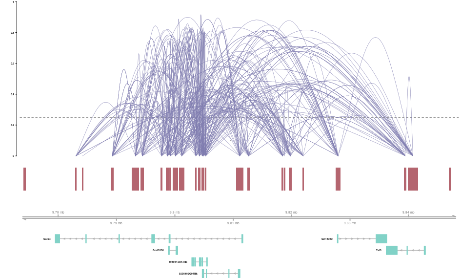
Cicero Connection可视化 有了peak之间共开放的可能性得分后,就可以画一些很酷的图了。用到的函数是plot_connections, 这个函数有很多参数,所以最终呈现结果取决于你的参数调整 。
获取基因组注释信息
1
2
3
4
5
6
7
8
9
temp <- tempfile() download.file("ftp://ftp.ensembl.org/pub/release-65/gtf/mus_musculus/Mus_musculus.NCBIM37.65.gtf.gz", temp) gene_anno <- rtracklayer::readGFF(temp) unlink(temp) gene_anno$chromosome <- paste0("chr", gene_anno$seqid) gene_anno$gene <- gene_anno$gene_id gene_anno$transcript <- gene_anno$transcript_id gene_anno$symbol <- gene_anno$gene_name
除了从GFF文件中提取外,还可以利用txdb提取转录本位置信息
举例子,下面的函数就是绘制染色体上"chr2:9773451-9848598的共开放情况,
1
2
3
4
5
plot_connections(conns, "chr2", 9773451, 9848598, gene_model = gene_anno, coaccess_cutoff = .25, connection_width = .5, collapseTranscripts = "longest" )
假如之前用的全基因组来算connections,那么这一步也会很久才能出图,所以建议先自己提取部分数据,这样子作图的速度就会快很多(因为源代码没有优化好矩阵过滤)
1
2
3
4
5
6
7
8
9
10
conns_sub <- conns[conns_matrix[,1] == "chr2" & as.numeric(conns_matrix[,2]) > 8000000 & as.numeric(conns_matrix[,2]) < 10000000 , ] plot_connections(conns_sub, "chr2", 9773451, 9848598, gene_model = gene_anno, coaccess_cutoff = .25, connection_width = .5, collapseTranscripts = "longest" )
计算基因活跃度得分 在启动子区的开放度并不是基因表达很好的预测子。使用Cicero links,我们就能得到启动子和它相关的远距位点的总体开放情况。这种区域间开放度联合得分和基因表达的相关度更高。作者称之为基因活跃度得分 (Cicero gene activity score)。 可以用两个函数进行计算
build_gene_activity_matrix函数接受CDS和Cicero connection list作为输入,返回一个标准化的基因得分。注意 , CDS必须在fData 表中有一列”gene”, 如果该peak在启动子区就用对应的基因名进行注释, 否则为NA. 我们可以用annotate_cds_by_site进行注释。
build_gene_activitity_matrix是未标准化的数据。需要用normalize_gene_activities进行标准化。如果你想比较不同数据集中部分数据的基因活跃度得分, 那么所有的gene activity 部分数据都需要一起标准化。如果只是想标准化其中一个数据集,那么传递一个结果即可。normalize_gene_activities也需要一个每个细胞所有开放位点的命名向量。这存放在CDS对象中的pData,在num_genes_expressed列。
可能还是不是明白,看代码吧。
第一步,是用annotate_cds_by_site对CDS对象进行注释在启动子区域的peak。
我们先从GFF文件中提取启动子的位置,也就是每个转录本的第一个外显子
1
2
3
4
5
6
7
8
9
10
11
12
13
14
15
16
17
18
19
20
21
22
23
24
# 分别提取正链和负链的注释, 仅保留第一个外显子 pos <- subset(gene_anno, strand == "+") pos <- pos[order(pos$start),] # remove all but the first exons per transcript pos <- pos[!duplicated(pos$transcript),] # make a 1 base pair marker of the TSS pos$end <- pos$start + 1 neg <- subset(gene_anno, strand == "-") neg <- neg[order(neg$start, decreasing = TRUE),] # remove all but the first exons per transcript neg <- neg[!duplicated(neg$transcript),] neg$start <- neg$end - 1 # 合并正链和负链 gene_annotation_sub <- rbind(pos, neg) # 只需要4列信息 gene_annotation_sub <- gene_annotation_sub[,c("chromosome", "start", "end", "symbol")] # 第四列命名为gene names(gene_annotation_sub)[4] <- "gene"
用annotate_cds_by_site对cds按照gene_annotation_sub注释。会多处两列,overlap和gene。
1
2
input_cds <- annotate_cds_by_site(input_cds, gene_annotation_sub) tail(fData(input_cds))
第二步: 计算未标准化的基因活跃度得分
1
2
3
4
5
6
# generate unnormalized gene activity matrix unnorm_ga <- build_gene_activity_matrix(input_cds, conns) # 过滤全为0的行和列 unnorm_ga <- unnorm_ga[!Matrix::rowSums(unnorm_ga) == 0, !Matrix::colSums(unnorm_ga) == 0]
第三步: 标准化基因活跃度得分
1
2
3
4
5
6
# 你需要一个命名列表 num_genes <- pData(input_cds)$num_genes_expressed names(num_genes) <- row.names(pData(input_cds)) # 标准化 cicero_gene_activities <- normalize_gene_activities(unnorm_ga, num_genes)
如果你有多个数据集需要进行标注化,那你就需要传递一个列表给normalize_gene_activities, 并且保证num_genes里包括所有数据集中的所有样本。
1
2
3
4
5
# if you had two datasets to normalize, you would pass both: # num_genes should then include all cells from both sets unnorm_ga2 <- unnorm_ga cicero_gene_activities <- normalize_gene_activities(list(unnorm_ga, unnorm_ga2), num_genes)
标注化后的基因活跃度得分在0到1之间,
第四步: 在UMAP上可视化基因得分。由于值比较小,要先扩大1000000倍,即log2(GA * 1000000 + 1),这样子在可视化的时候比较好看。
1
2
3
4
5
6
7
8
9
10
11
12
13
14
15
16
17
18
19
20
plot_umap_ga <- function(cds, cicero_gene_activities, gene, dotSize = 1, log = TRUE){ #umap_df <- as.data.frame(colData(cds)) umap_df <- as.data.frame(reducedDims(input_cds)$UMAP) colnames(umap_df) <- c("UMAP1","UMAP2") gene_pos <- which(row.names(cicero_gene_activities) %in% gene) umap_df$score <- log2(cicero_gene_activities[gene_pos,] * 1000000 + 1) if (log){ umap_df$score <- log(umap_df$score + 1) } p <- ggplot(umap_df, aes(x=UMAP1, y=UMAP2)) + geom_point(aes(color=score), size = dotSize) + scale_color_viridis(option="magma") + theme_bw() return(p) }
拟时序分析 这部分的分析其实比较简单,因为仅仅是将feature从mRNA变成了peak而已。步骤如下
数据预处理
数据降维
细胞聚类
轨迹图学习
在拟时间上对细胞进行排序
代码如下
1
2
3
4
5
6
7
8
9
10
11
12
13
14
15
16
# 读取数据 temp <- textConnection(readLines(gzcon(url("http://staff.washington.edu/hpliner/data/kidney_data.txt.gz"))))set.seed(2017) input_cds <- estimate_size_factors(input_cds) #1 数据预处理 input_cds <- preprocess_cds(input_cds, method = "LSI") #2 降维 input_cds <- reduce_dimension(input_cds, reduction_method = 'UMAP', preprocess_method = "LSI") #3 细胞聚类 input_cds <- cluster_cells(input_cds) #4 轨迹图学习 input_cds <- learn_graph(input_cds) #5 对细胞进行排序 input_cds <- order_cells(input_cds, root_cells = "GAGATTCCAGTTGAATCACTCCATCGAGATAGAGGC")
最后可视化
1 plot_cells(input_cds, color_cells_by = "pseudotime")
差异开放分析 当你的细胞在拟时间中排列之后,你可能会想知道基因组哪些区域会随着时间发生变化。
如果你已经知道哪些区域会随着时间发生变化,你可以用plot_accessibility_in_pseudotime进行可视化
1
2
3
4
input_cds_lin <- input_cds[,is.finite(pseudotime(input_cds))] plot_accessibility_in_pseudotime(input_cds_lin[c("chr1_3238849_3239700", "chr1_3406155_3407044", "chr1_3397204_3397842")])
当然我们也可以从头分析. 先用aggregate_by_cell_bin对细胞根据相似度进行聚合
1
2
3
4
# First, assign a column in the pData table to umap pseudotime pData(input_cds_lin)$Pseudotime <- pseudotime(input_cds_lin) pData(input_cds_lin)$cell_subtype <- cut(pseudotime(input_cds_lin), 10) binned_input_lin <- aggregate_by_cell_bin(input_cds_lin, "cell_subtype")
之后用Monocle3的fit_models函数寻找差异开发的区域。
1
2
3
4
5
6
7
8
9
# For speed, run fit_models on 1000 randomly chosen genes set.seed(1000) acc_fits <- fit_models(binned_input_lin[sample(1:nrow(fData(binned_input_lin)), 1000),], model_formula_str = "~Pseudotime + num_genes_expressed" ) fit_coefs <- coefficient_table(acc_fits) # Subset out the differentially accessible sites with respect to Pseudotime pseudotime_terms <- subset(fit_coefs, term == "Pseudotime" & q_value < .05) head(pseudotime_terms)
参考资料