2019年发表在Nature上的文章【The single-cell transcriptional landscape of mammalian organogenesis】在方法部分提到,使用NNLS(non-negative linear-square)回归的方法分析两个细胞图谱数据集中相关细胞类型。
这个方法,在我搜索的中文教程中都没有出现过,所以这里以两个pbmc的数据集为例进行介绍,如何复现文章的方法。
10x的细胞数据集的预处理部分不做过多介绍, 如下代码以10x官网提供的数据为例
1 2 3 4 5 6 7 8 9 10 11 12 13 14 15 library( Seurat) pbmc.data <- Read10X_h5( "./data/10x/10k_PBMC_3p_nextgem_Chromium_X_filtered_feature_bc_matrix.h5" ) seu.obj <- CreateSeuratObject( counts = pbmc.data, project = "pbmc10k" , min.cells = 3 , min.features = 200 ) library( dplyr) seu.obj <- seu.obj %>% Seurat:: NormalizeData( verbose = FALSE ) %>% FindVariableFeatures( selection.method = "vst" ) %>% ScaleData( verbose = FALSE ) %>% RunPCA( pc.genes = seu.obj@ var.genes, npcs = 100 , verbose = FALSE ) %>% FindNeighbors( dims = 1 : 10 ) %>% FindClusters( resolution = 0.5 ) %>% RunUMAP( dims = 1 : 10 )
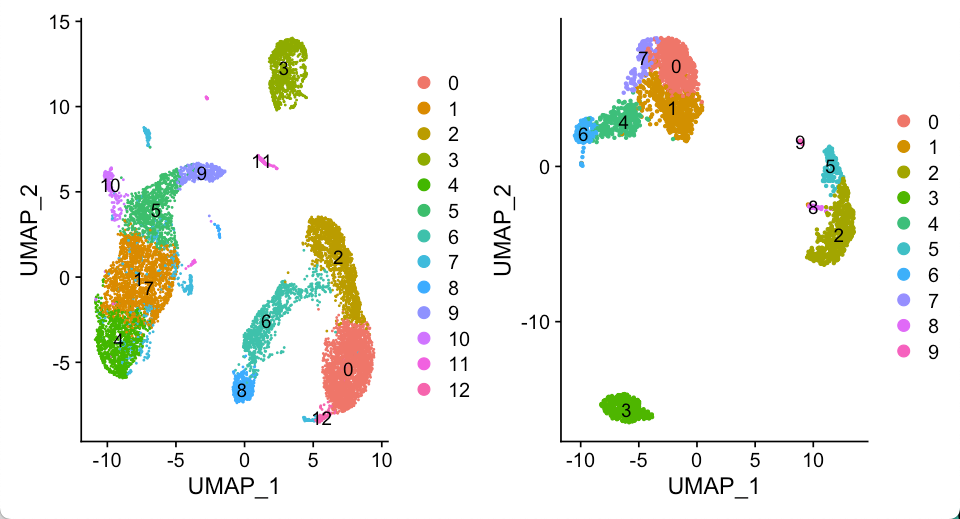
相同的处理流程我们应用到Seurat 3k教程 里. 最终我们得到两个Seurat对象
seu.obj1: 10x的10k pmbc
seu.obj2: 10x的3k pbmc
基本上看多了PBMC数据的UMAP结果,大概就能通过UMAP的拓扑结构推断不同的细胞类型,比如说两个数据集的cluster3, 肯定都是B细胞了。
接着,我们基于文章的描述来实现代码
第一步是对数据按照cluster进行合并,并进行标准化
To identify correlated cell types between two cell atlas datasets, we first aggregated the cell-type-specific UMI counts, normalized by the total count, multiplied by 100,000 and log-transformed after adding a pseudocount
1 2 3 4 5 6 7 8 9 10 11 12 13 shared_gene <- intersect( rownames( seu.obj) , row.names( seu.obj2) ) seu.obj.mat <- Seurat:: AggregateExpression( seu.obj, assays = "RNA" , features = shared_gene, slot = "count" ) $ RNA seu.obj.mat <- seu.obj.mat / rep ( colSums( seu.obj.mat) , each = nrow( seu.obj.mat) ) seu.obj.mat <- log10( seu.obj.mat * 100000 + 1 ) seu.obj.mat2 <- Seurat:: AggregateExpression( seu.obj2, assays = "RNA" , features = shared_gene, slot = "count" ) $ RNA seu.obj.mat2 <- seu.obj.mat2 / rep ( colSums( seu.obj.mat2) , each = nrow( seu.obj.mat2) ) seu.obj.mat2 <- log10( seu.obj.mat2 * 100000 + 1 )
第二步是筛选基因. 文章为了提高准确性,先根据目标数据集中给定细胞类型和整体细胞类型中位数的倍数变化,选择前200个;然后给根据目标数据集中给定细胞类型和其他细胞类型最大值的倍数变化,选择前200个,对两个结果进行合并。(我使用差异富集的marker的前100个,发现效果也差不多)
To improve accuracy and specificity, we selected cell-type-specific genes for each target cell type by (1) ranking genes on the basis of the expression fold-change between the target cell type versus the median expression across all cell types, and then selecting the top 200 genes; (2) ranking genes on the basis of the expression fold-change between the target cell type versus the cell type with maximum expression among all other cell types, and then selecting the top 200 genes; and (3) merging the gene lists from steps (1) and (2).
1 2 3 4 5 6 7 8 9 10 11 12 13 cluster <- 3 seu.obj.gene <- seu.obj.mat[ , cluster + 1 ] gene_fc <- seu.obj.gene / apply( seu.obj.mat, 1 , median) gene_list1 <- names ( sort( gene_fc, decreasing = TRUE ) [ 1 : 200 ] ) gene_fc <- seu.obj.gene / apply( seu.obj.mat[ , - ( cluster+ 1 ) ] , 1 , max ) gene_list2 <- names ( sort( gene_fc, decreasing = TRUE ) [ 1 : 200 ] ) gene_list <- unique( c ( gene_list1, gene_list2) )
第三步: 是在相关系数不为负的限制下,求解 $T_a = \beta_0a + \beta_{1a}M_b$. 其中 $M_b$ 是预测数据集的基因表达量, $\beta_{1a}$就是对应系数。
1
2
3
4
5
6
7
Ta <- seu.obj.mat[ gene_list, cluster+ 1 ] Mb <- seu.obj.mat2[ gene_list, ] library( lsei) solv <- nnls( Mb, Ta) corr <- solv$ x
这里算出预测数据集的cluster3系数最高,为0.93, 其他都是0.
第四步: 调换预测数据集和目标数据集,重新进行第二步和第三步
Similarly, we then switch the order of datasets A and B, and predict the gene expression of target cell type (Tb) in dataset B with the gene expression of all cell types (Ma) in dataset A.
1 2 3 4 5 6 7 8 9 10 11 12 13 14 15 seu.obj.gene <- seu.obj.mat2[ , cluster] gene_fc <- seu.obj.gene / apply( seu.obj.mat2, 1 , median) gene_list1 <- names ( sort( gene_fc, decreasing = TRUE ) [ 1 : 200 ] ) gene_fc <- seu.obj.gene / apply( seu.obj.mat2[ , - cluster] , 1 , max ) gene_list2 <- names ( sort( gene_fc, decreasing = TRUE ) [ 1 : 200 ] ) gene_list <- unique( c ( gene_list1, gene_list2) ) Ta <- seu.obj.mat2[ gene_list, cluster] Mb <- seu.obj.mat[ gene_list, ] solv <- nnls( Mb, Ta) corr2 <- solv$ x
第五步: 经过上面运算后,我们就得到对于数据集A中的各个细胞类型,数据集B各个细胞类型对应的回归系数,记作 $\beta_{ab}$ 以及对于数据集B中的各个细胞类型,数据集A各个细胞类型对应的回归系数, $\beta_{ba}$, 通过如下公式整合两个参数, $\beta = 2(\beta_{ab} + 0.01)(\beta_{ba} + 0.01)$
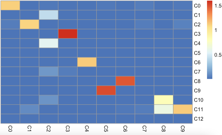
1 2 3 4 5 6 7 8 9 10 11 12 13 14 15 16 17 18 19 20 21 22 23 24 25 26 27 28 29 30 31 32 33 34 35 36 37 38 39 40 41 42 43 44 45 46 47 48 49 50 51 52 53 54 55 56 57 58 59 list1 <- list ( ) for ( cluster in seq( 1 , ncol( seu.obj.mat) ) ) { seu.obj.gene <- seu.obj.mat[ , cluster] gene_fc <- seu.obj.gene / apply( seu.obj.mat, 1 , median) gene_list1 <- names ( sort( gene_fc, decreasing = TRUE ) [ 1 : 200 ] ) gene_fc <- seu.obj.gene / apply( seu.obj.mat[ , - cluster] , 1 , max ) gene_list2 <- names ( sort( gene_fc, decreasing = TRUE ) [ 1 : 200 ] ) gene_list <- unique( c ( gene_list1, gene_list2) ) Ta <- seu.obj.mat[ gene_list, cluster] Mb <- seu.obj.mat2[ gene_list, ] solv <- nnls( Mb, Ta) corr <- solv$ x list1[[ cluster] ] <- corr } list2 <- list ( ) for ( cluster in seq( 1 , ncol( seu.obj.mat2) ) ) { seu.obj.gene <- seu.obj.mat2[ , cluster] gene_fc <- seu.obj.gene / apply( seu.obj.mat2, 1 , median) gene_list1 <- names ( sort( gene_fc, decreasing = TRUE ) [ 1 : 200 ] ) gene_fc <- seu.obj.gene / apply( seu.obj.mat2[ , - cluster] , 1 , max ) gene_list2 <- names ( sort( gene_fc, decreasing = TRUE ) [ 1 : 200 ] ) gene_list <- unique( c ( gene_list1, gene_list2) ) Ta <- seu.obj.mat2[ gene_list, cluster] Mb <- seu.obj.mat[ gene_list, ] solv <- nnls( Mb, Ta) corr <- solv$ x list2[[ cluster] ] <- corr } mat1 <- do.call( rbind, list1) mat2 <- do.call( rbind, list2) beta <- 2* ( mat1 + 0.01 ) * t( mat2+ 0.01 ) row.names( beta) <- paste0( "C" , 1 : nrow( beta) - 1 ) colnames( beta) <- paste0( "C" , 1 : ncol( beta) - 1 ) pheatmap:: pheatmap( beta, cluster_rows = FALSE , cluster_cols = FALSE )
结果如下:
观察发现: 3k数据集UMAP上邻居的C4,6对应10k数据集的C6和C8也是临近关系, 说明基于NNLS的预测方法,也是相对比较准确。
当然文章也通过对多个数据集的相互比较验证了这个分析方法。
For validation, we first applied cell-type correlation analysis to independently generated and annotated analyses of the adult mouse kidney (sci-RNA-seq component of sci-CAR19 versus Microwell-seq). We subsequently compared cell subclusters from this study (with detected doublet-cell ratio ≤10%) to fetus-related cell types (those with annotations including the term ‘fetus’) from the Microwell-seq-based MCA. A similar comparison was performed against cell types annotated in BCA.
但是,文章并没有解释他可以用NNLS回归的方法做标记的迁移,鉴于他没有引述参考文章,我们可以认为这是作者第一次提出的标记迁移思路。所以,不妨让我做一些推测吧。
我们比较耳熟能详的分析是,线性回归里面的最小二乘法,也就是给定两组变量a和b, 通过最小二乘的方法求解a = bx + c中的系数x和c. 那么,假设存在三个细胞类型A, B,C. 其中A和B是同一类型,A和C不是同一类型。对于同一种细胞类型的两个数据,只不过由于实验,测序和分析等各种因素,导致基因表达值并不相同,但是存在着一定关联。我们可以通过求解 A = Bx + Cy 中的系数x, y,通过比较系数来评估A和哪个细胞类型最类似。进一步, 显然我们不能让一个细胞类型的贡献为负,最少是无作用,也就是0, 因此我们就得 限定系数不为负 ,也就是非负最小二乘(non-negative linear square, NNLS)回归。